
Sparse Error Correction via Logan Phenomenon [python]
Published:
Python demo of Figure 2.16 Sparse Error Correction via Logan’s Phenomenon from High-Dimensional Data Analysis with Low-Dimensional Models - John Wright, Yi Ma, Page 65
Problem
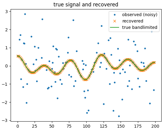
B is a matrix with columns from low frequency basis from Fourier Discrete Transform matrix, we want to recovery original noisy-free signal x from observation y.
\[\begin{eqnarray} \min || y - x||_1 \\ s.t. \ x \in col(B) \end{eqnarray}\]in this demo, Discrete Cosine Transform is used, to avoid complex number in basis pursuit. The author does not know how to do with complex space yet.
result
signal
error
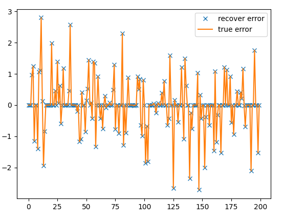
try to change the Omega and sparsity of the following code to see when the error cannot be separated.
code
from IPython.core.getipython import get_ipython      # for %matplotlib
get_ipython().run_line_magic('matplotlib', 'widget') # install pip install ipympl

import numpy as np
import matplotlib.pyplot as plt
from scipy.fftpack import dct

def lasso(A, y):
    _, n = A.shape

    # initialize
    x = np.random.randn(n, 1)

    # lr = 0.001
    B = A.T @ np.linalg.inv(A @ A.T)

    for i in range(1, 20000):
        # print(i)
        dx = np.sign(x)
        lr = 1/i
        x = x - lr*dx
        x = x - B @ (A@x - y)

        # err.append(np.linalg.norm(x-x0, 1))

    return x

m = 200

# F = np.matrix(np.fft.fft(np.eye(m))) / np.sqrt(m)     # got a complex basis, and I do not know how to solve it by subgradient projection

F = np.matrix(dct(np.eye(m)))  # strange: the first column has a large norm
F = F / np.linalg.norm(F, axis=0)

# for fct F is conjugate horizontal symmetric in 2,...,N columns, see comment at the end of this scripts
# for dct F seems like to a a half of the full fct matrix

# get low freqencies: B matrix
Omega = 6
B = F[:, :2*Omega]  # low frequencies
n = B.shape[1]
print('got {} low frequencies basis'.format(n))

# get high frequencies: A matrix (span the left null spaces)
A = F[:, 2*Omega:].H
assert(np.allclose(A @ B, 0))

# plt.figure(); plt.imshow(np.hstack([F.real, F.imag]), cmap='gray')
plt.figure(); plt.imshow(np.hstack([B, np.zeros([m, 3]), A.H.real]), cmap='gray')

# signal and error
x0 = np.random.randn(n, 1)
e0 = np.random.randn(m, 1)

sparsity = 100   # non zeros
zero_i = np.random.choice(m, m - sparsity, replace=False)
e0[zero_i] = 0.0

# sparsity is the support of error in Logan's Theorem?
print('support*Omega:', sparsity * Omega)

s0  = B @ x0     # the signal
y = s0 + e0

# let's see some high frequency signal basis
plt.figure(); plt.plot(F[:, -10], '.-')
# and the bandlimited signal we want to restore or separate
plt.figure(); plt.plot(s0, '.'); plt.title('andlimited signal to recover')
plt.plot(y, '.'); plt.title('true signal with error')
# what does high frequencies look like?
# plt.figure(); plt.plot(A.T[:, -x0.shape[0]:] @ x0, '.-')


# let's find e
y_hat = A @ y

e = lasso(A, y_hat)
s = y - e

print(np.linalg.norm(e-e0, 1) / np.linalg.norm(e0, 1))

plt.figure(); plt.plot(y, '.'); plt.plot(s, 'x'); plt.plot(s0, '-'); plt.title('true signal and recovered'); plt.legend(['observed (noisy)', 'recovered', 'true bandlimited'])

plt.figure(); plt.plot(e, 'x'); plt.plot(e0, '-'); plt.legend(['recovered error',  'true error'])